1. Introduction to PCA in SPSS
Principal Component Analysis (PCA) is a widely used technique for dimensionality reduction in SPSS. Dimensionality reduction is another ML data preprocessing activity besides feature selection. PCA reduces input data dimensionality through statistical techniques by transforming correlated variables into a set of uncorrelated variables. These have a smaller dimension but still retain most of the data’s variance.
Similar to feature selection, PCA simplifies the ML model’s input data for both training and inference. Removing data redundancy is valuable since it reduces resources for storing and processing extra data and improves processing speed. Additionally, redundant data removal reduces overfitting by eliminating noise and irrelevant information from the input data.
SPSS is an existing commercial software package that provides a built-in PCA tool with a guided interface providing access. Therefore, ML engineers can readily use this for PCA without any additional coding, speeding up development time. Social sciences widely adopt this because of its robust statistical tools in psychology and social science. Additionally, it has well-formatted output for academic reporting and publication standards.
This tutorial will demonstrate how to run PCA within SPSS through clear, step-by-step instructions. It will go through the entire PCA processing from data preparation through to interpreting the output.
2. What is PCA? (Brief Refresher)
What makes PCA in SPSS so useful is that it helps to uncover hidden patterns in data. Through dimensionality reduction, it identifies the underlying variables that explain most of the variance. Therefore, it transforms correlated variables into variables that are orthogonal and independent of each other. Subsequently, fewer dimensions allow for more efficient data visualization and exploration. Additionally, it reduces dataset complexity but still keeps the structure that contains most of the overall information. PCA is most effective when two or more of the input variables have a high correlation, carrying overlapping or redundant information. Therefore, analysts can focus on the most significant components and filter out less impactful variations.
There are several key concepts with PCA in SPSS, including components, eigenvalues, and variance explained.
Components are the uncorrelated variables that Principal Component Analysis (PCA) creates from the original dataset. Each component is a linear combination of the original variables that captures a specific portion of the dataset’s variance.
The next concept is eigenvalue; each component has an eigenvalue associated with it. An eigenvalue indicates the variance that its corresponding component captures. The higher the eigenvalue, the more the associated component captures the dataset’s total variability.
Variance explained refers to the proportion of the dataset’s total variance captured by each component. Therefore, we use PCA to create the components that explain most of the variance and eliminate those with minimal contribution.
Now that we’ve reviewed key concepts, let’s walk through how to perform PCA in SPSS step by step.
3. Preparing Your Data in SPSS for Effective PCA
Although dimensionality reduction using PCA in SPSS is a data preprocessing activity, you need pre-steps in your workflow.
Input data must satisfy PCA data requirements for it to apply any effective dimensionality reduction. We can only apply metric variables to PCA that are numerical variables that have meaningful numerical values and consistent units. They are either measured on an interval or ratio scale. Also, these variables must be continuous and not categorical or discrete. Additionally, we need to properly transform any nominal or ordinal variables. Otherwise, they are not suitable for PCA.
PCA also assumes complete data, making it critical to check for and handle any missing values before any dimensionality reduction. Otherwise, these missing values can distort the component structure and generate biased results. Since PCA uses statistical calculations, the presence of outliers disproportionately influences the principal components. Please refer to our guide on identifying missing data.
Scaling is just as important to PCA as it is to model training, where larger numerical ranges can dominate and distort results. In this case, these variables can dominate principal components. SPSS provides functions that can standardize each variable to have a mean of zero and a standard deviation of one.
Since PCA is statistically based, larger sample sizes work better than smaller ones to produce reliable results. Empirical evidence points to having at least 5 to 10 observations per variable for reliable PCA results.
4. How to Run PCA in SPSS (Step-by-Step)
Once we have adequately prepared our data, we can now apply PCA in SPSS to reduce its dimensionality.
SPSS has a graphical user interface (GUI) that makes usability one of its key strengths. SPSS also includes a command line interface, which is useful for reproducibility and scripting workflows once you’re more advanced. When starting with SPSS, it is best to use its GUI until one has attained mastery of it. A mock-up of SPSS is provided below.
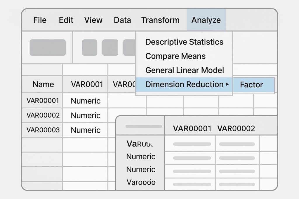
Start the SPSS GUI so that we can properly configure SPSS for us to run its Principal Component Analysis (PCA). Next, we need to open our dataset in SPSS prior to running the PCA process. When the dataset is opened in SPSS, we click on the “Analyze” menu. This is at the top of SPSS as shown in the mock-up. Then, we hover over “Dimension Reduction” in the dropdown menu and select “Factor” from the submenu. This will open the PCA setup window.
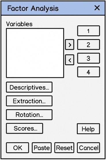
Now that we are in the Factor Analysis window, we want to select the variables we want to include in PCA. Remember to only select continuous metric variables; PCA will not handle any other types of variables. We select our variables by using the arrow button to move our chosen variables into the analysis box.
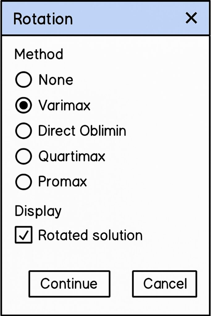
“Varimax rotation” helps to make components easier to interpret by clarifying variable loadings. To select this, click the “Rotation” button in the “Factor Analysis” dialog box. In the “Rotation Method” section, select “Varimax” as the default orthogonal option. Also, you can check “Display rotated solution” to view the output. Click “Continue” to return to the main “Factor Analysis” window.
Configure Extraction
Once we have selected our variables, we are ready to perform principal component analysis (PCA). We click the Extraction button in the Factor Analysis dialog, which will open up the Extraction dialog as shown below.
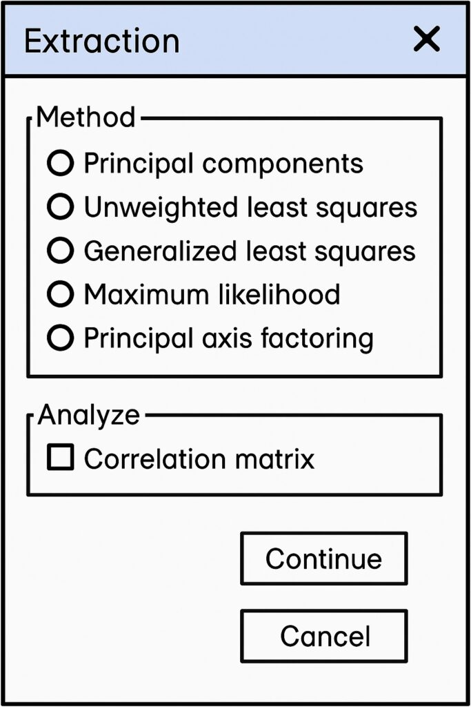
When the Extraction dialog is opened, we select the “Principal components” radio button to select our extraction method. This updates the “Extraction” dialog as shown below.
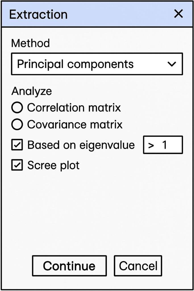
In order to visualize the variance, select the “Scree plot” checkbox. Also, ensure that the eigenvalues are greater than one by selecting the “Based on eigenvalue” checkbox. Leave the textbox with the default “1.0”; here it is shown as “> 1” to aid in understanding. Selecting eigenvalues greater than one follows the Kaiser criterion, which retains only the components that explain substantial variance.
Next, click the “Continue” button, and we will return to the main SPSS window.
After completing the extraction settings, you’re now ready to run PCA by clicking “OK” in the Factor Analysis window.
5. Interpreting PCA Output in SPSS
Once we have run PCA in SPSS, we now want to interpret the output, which includes:
- Communalities Table
- Total Variance Explained Table
- Scree Plot
- Component Matrix
- Rotated Component Matrix
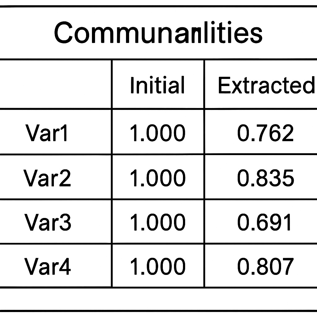
Communalities Table
The Communalities Table shows how well each variable is explained by the retained components. In other words, the amount of variance each variable shares with the extracted components. It shows both the initial and extracted communalities that exist for each variable. PCA always sets the initial communality to 1.0 because it represents total variance. The extracted communalities indicate the proportion of a variable’s variance that is explained by the retained components. Variables that have higher communalities suggest that they are better represented by the extracted components.
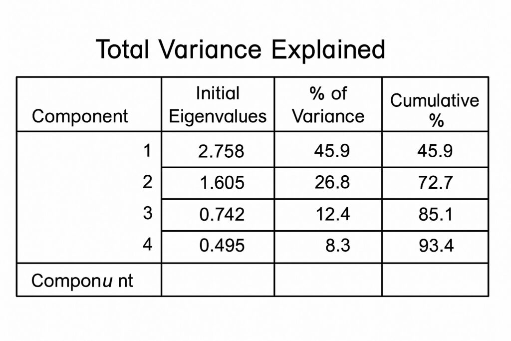
Total Variance Explained Table
Next is the Total Variance Explained Table that summarizes the variance that each principal component accounts for. This includes the eigenvalues and the percentage of the variable that each component explains. Using the Kaiser criterion, PCA typically retains components that have eigenvalues greater than one. The cumulative variance shows how many components capture a sufficient amount of total variability. Hence, components with higher eigenvalues indicate that they explain a greater proportion of the dataset’s overall variance.
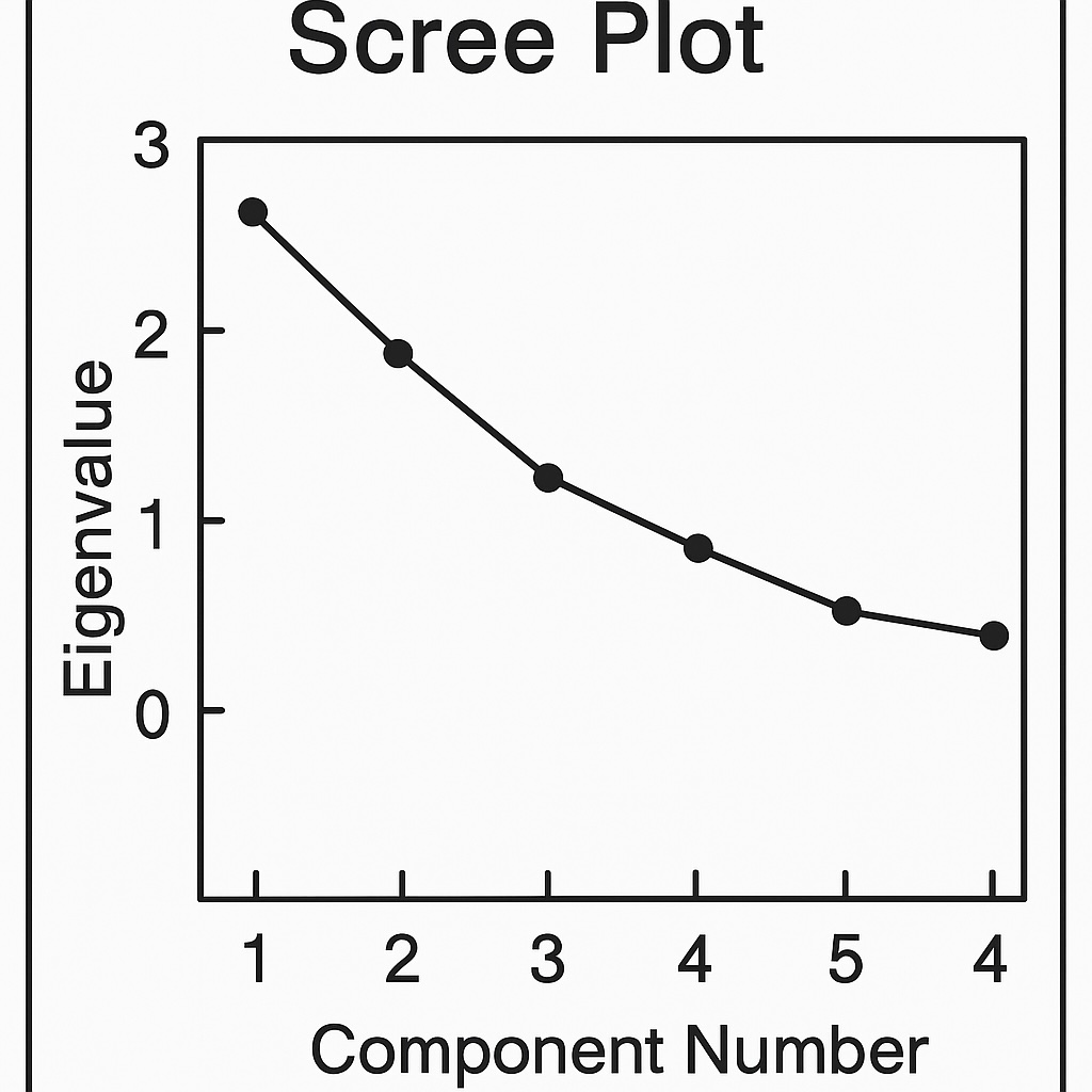
Scree Plot
The previous tables display components and their variance in a tabulated format. In contrast, the Scree Plot presents this information in a graphical format. The graphical format aids in better understanding how much each component contributes to the dataset variance. The “elbow” point in the graph where the slope levels off suggests the optimal number of components. Components before the elbow usually capture meaningful variance. In contrast, those after contribute little and should be excluded from the final model.
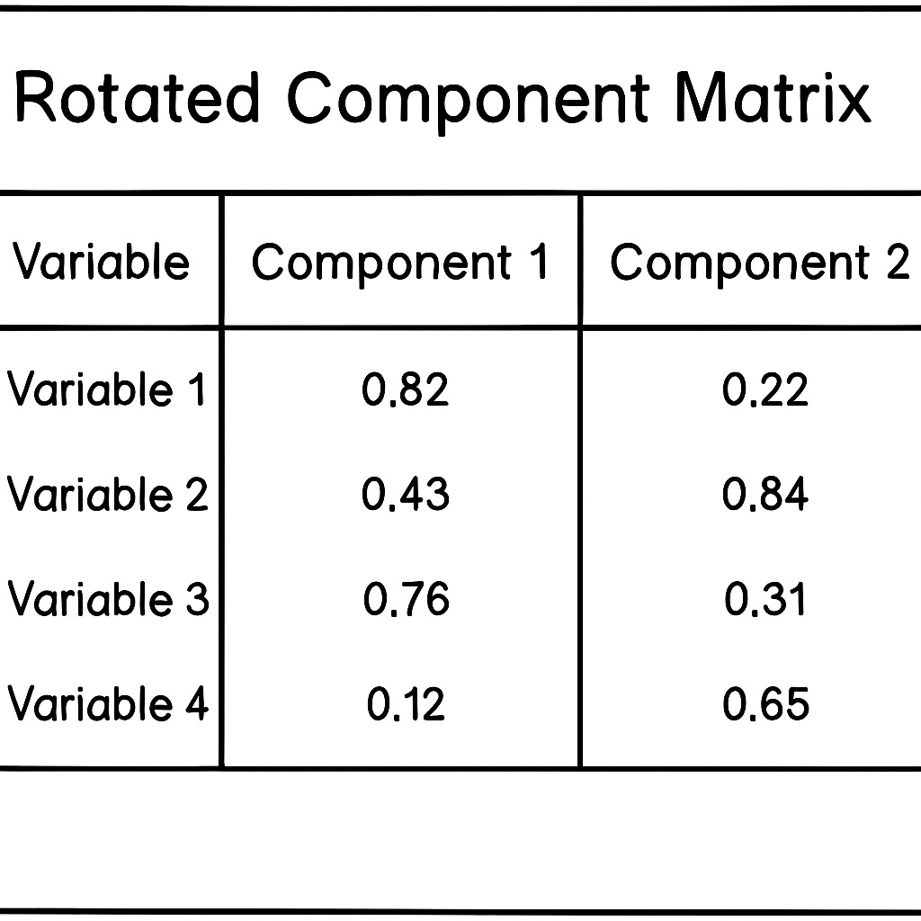
Rotated Component Matrix
The Rotated Component Matrix shows how strongly each variable loads onto each component. This is rotated to simplify the structure and make the components more straightforward to interpret. Here, higher absolute loadings usually indicate a stronger relationship between the variable and the component. In other words, variables with higher loadings on the same component suggest they share an underlying factor. An empirical rule of thumb stipulates that loadings are meaningful when above 0.4.
Practical Tips
There are a couple of practical tips when naming components. When naming components, it is good practice to name them based on the variables that load most strongly onto them. Additionally, use clear, descriptive labels that reflect the shared theme or pattern among high-loading variables.
6. PCA in SPSS Use Cases and Benefits
After considering how to run PCA in SPSS, we will now consider an actual example where we can apply this. A suitable use case is surveys that use Likert-scale items measuring related concepts. Likert-scale items quantify subjective perceptions into numerical values. An example is satisfaction, quantified from 1 to 5, where 1 represents the least satisfied and 5 represents the most satisfied.
Principal Component Analysis (PCA) can group these correlated items into a few underlying factors. Therefore, applying PCA reduces complexity by summarizing 10 items into 2 or 3 core dimensions. These core components will then help identify dominant themes, such as satisfaction, trust, or engagement.
From this, there are several practical applications including psychology, consumer preference, and educational satisfaction. Applying PCA to psychological tests will help reduce multiple questionnaire items into a set of core traits or constructs. For consumer research, PCA can identify key preference dimensions from product rating surveys. With education, it can simplify student satisfaction data into factors like teaching quality or course relevance.
PCA in SPSS’s most significant contribution is reducing noise and simplifying reporting. The most important contribution is filtering out redundant or low-variance variables that provide little to no helpful information. PCA improves interpretability by condensing complex datasets into a few key components that aid in understanding. Finally, it improves presentation when there are simplified outputs resulting in clear, focused visualization and reports.
7. Common PCA in SPSS Mistakes to Avoid
We can still misuse PCA in SPSS, and there are several common pitfalls that can trip us up.
For PCA to work correctly, we need to transform categorical variables into numeric forms prior to using PCA. However, we should avoid one-hot encoding since it can introduce sparsity and high dimensionality, defeating the purpose. When transforming categorical data, we need to proceed cautiously and interpret the results accordingly. This is because PCA is most effective when applied to continuous variables.
Another pitfall is when low communality variables do in fact reflect unique variances, and their removal can discard valuable information. While they may not align with the extracted components, it does not mean they lack relevance. In other words, do not remove variables solely on low communality.
PCA in SPSS that generates too many components can reintroduce noise and reduce clarity. Additionally, we can derive misleading conclusions when overinterpreting small variance components. Also, we complicate reporting without any meaningful insight when we have too many components.
We can also skip rotation, which makes component interpretation harder due to mixed loadings. Additionally, unrotated solutions can often obscure clear patterns among variables.
8. Conclusion & Further Resources
We have explored dimensionality reduction through PCA in SPSS to simplify models and derive key insights in these models. Simplification reduces redundancy, which makes models harder to understand through unnecessary noise. This leads to less complicated visualizations that better highlight the model’s influencing factors, aiding in understanding. The models themselves are cleaner, leading to analytics that are better placed to derive meaningful insight and make better data-driven decisions.
Students in this field can purchase SPSS at student rates, allowing them to experiment and practice with real datasets. Hands-on learning will greatly enhance the theory taught on this powerful statistical technique.
9. Further Reading
For those looking to deepen their understanding of PCA, SPSS, and applied statistics, consider these highly regarded resources:
- Discovering Statistics Using IBM SPSS Statistics (5th Edition) by Andy Field
A comprehensive, humorous, and reader-friendly guide covering statistics and SPSS, with practical examples on PCA and factor analysis. - An Introduction to Statistical Learning with Applications in R (2nd Edition) by Gareth James, Daniela Witten, et al.
Offers a gentle yet thorough introduction to machine learning techniques, including dimensionality reduction, with conceptual clarity and R-based examples. - Applied Multivariate Statistical Analysis (6th Edition) by Richard A. Johnson & Dean W. Wichern
A classic textbook that provides mathematical depth on PCA, factor analysis, and multivariate statistics, widely used in academic settings.
Affiliate Disclosure
This post contains affiliate links. If you purchase through these links, AI Cloud Data Pulse may earn a small commission at no extra cost to you. We only recommend resources we trust and believe will add value to our readers.
10. References
IBM SPSS PCA Documentation
Link to the official IBM SPSS documentation for factor analysis or PCA setup.
➤ https://www.ibm.com/docs/en/spss-statistics
Wikipedia – Principal Component Analysis
Offers a concise mathematical and conceptual overview.
➤ https://en.wikipedia.org/wiki/Principal_component_analysis
Laerd Statistics – PCA in SPSS
A trusted academic-style walkthrough that complements this guide.
➤ https://statistics.laerd.com/