1. Introduction to PCA Using Scikit-Learn
PCA using Scikit-Learn helps simplify data, which is a crucial step in data preprocessing within the Machine Learning (ML) workflow. Data preprocessing activities include cleaning data, removing errors, and simplifying it. Simplified data results in less complex ML models that are more efficient and require fewer computing resources. Dimensionality reduction is a data simplification technique that reduces the number of features while keeping essential information.
Previously, we covered how feature selection simplifies data by selecting only the most relevant features. Dimensionality reduction complements this by retaining all features while transforming them into a lower-dimensional space, thereby further simplifying the data. High-dimensional data often has noise, redundancy, and multicollinearity, which the dimensionality reduction helps to remove. Another benefit is that it is easier to visualize data with fewer dimensions, especially in 2D or 3D. This is where we can make use of PCA using Scikit-learn.
PCA is a dimensionality reduction technique that fits well into an ML workflow, preserving overall data structure while reducing complexity. It achieves this by projecting data onto orthogonal components, allowing for more stable model training. PCA uncovers hidden patterns, so the model doesn’t have to learn them from scratch.
PCA using Scikit-learn makes it easy for developers to implement PCA with minimal lines of code. It also enables them to seamlessly integrate PCA into ML pipelines.
This post provides an introduction to PCA concepts, along with a hands-on implementation of the PCA algorithm. Additionally, we will survey the benefits of PCA along with common pitfalls and will consider real-world examples.
2. What is PCA?
Principal Component Analysis (PCA) using Scikit-learn reduces the number of variables in a dataset without sacrificing important information. This is achieved by identifying the key directions where the data varies the most, and it refers to these as principal components. Hence the name principal component analysis. These components become the new features that the PCA algorithm creates from combinations of the original features. This results in projecting the dataset onto a lower-dimensional space, revealing its underlying structure. Therefore, it retains the most meaningful information but removes noise and redundancy.
Deriving principal components from existing features reduces their overlap when it combines highly correlated variables into a single component. This also eliminates multicollinearity within these features, which helps to improve model stability. Another benefit is that it highlights dominant trends and relationships that are not easily read in the raw data. Hence, PCA reveals the dataset’s true structure beneath its surface complexity by revealing its strongest patterns.
The key concept behind principal component analysis is transforming data into fewer dimensions while keeping its variances. By streamlining this representation, it allows ML models to focus on the most significant variations in the dataset. This enhances model performance by reducing the dimensionality burden without losing essential information. This makes PCA with Scikit-learn an invaluable tool for ML workflows.
3. When to Use PCA with Scikit-learn
There are certain scenarios that are better suited to applying PCA using Scikit-learn than others.
Datasets that have high dimensionality with multicollinearity are usually the best candidates for PCA. These datasets are more likely to contain features that are strongly correlated with each other, making them ripe for PCA. Crucially, multicollinearity within datasets can distort machine learning models and inflate variance in their predictions. Additionally, when redundant features dominate the data, it is more challenging to interpret model outputs. Therefore, PCA can address datasets with these problems by combining correlated features into independent components.
PCA preprocessing using Scikit-Learn is best suited for classification and clustering ML models and less suited for tree-based models. It is also poorly suited for linear regression models, except for very high-dimensional cases. PCA helps clustering models by reducing noise and highlighting meaningful structure in datasets. Clustering algorithms like K-means can form tighter, more distinct groups with reduced dimensionality that PCA provides. PCA also improves the performance of classification models by removing redundant and correlated features. Additionally, classification models are faster and more efficient when PCA simplifies the feature space.
Alongside ML models, PCA helps data scientists and data engineers to perform exploratory data analysis. They are able to visualize high-dimensional data in two or three dimensions. Also, when they plot the first few principal components, they can quickly see clusters, trends, or outliers. These are often difficult or impossible to see in the raw feature space.
An important point to note is that PCA is unsupervised, and ML workflows should only apply it after scaling.
4. How PCA Works: Core Concepts
Now that we’ve explained what PCA using Scikit-learn does and when to use it, let’s walk through how it works step by step. PCA follows a sequence of steps when transforming a dataset into principal components, and we describe these below.
The first action that PCA takes is mean-centering and standardization of each feature. The first is to shift each feature so that its average value is zero. It then scales each feature so that its variance is one, allowing fair comparisons across each dimension. It is important to scale data prior to PCA since it assumes data is on the same scale. Otherwise, features with larger ranges can dominate the principal components.
The following action is that PCA calculates the covariance matrix of the standardized data from the previous step. This illustrates how the features within the dataset vary in relation to one another. PCA then uses eigen decomposition to resolve this matrix into eigenvalues and eigenvectors that reveal key data directions. Eigenvectors represent the axes along which the data varies the most, which become the principal components. Meanwhile, eigenvalues represent the degree of variance that each corresponding principal component captures.
The algorithm uses the Scree plot to select which components to keep based on the explained variance ratio. The Scree plot illustrates the variance explained by each principal component, with the “elbow point” indicating where additional components contribute diminishing returns. The components above the elbow point combined contain the dataset’s most meaningful variance, while those below contain the least significant variance. Therefore, the algorithm selects components above the elbow point for the transformed dataset.
5. Step-by-Step: PCA Using Scikit-Learn
Now that we have taken a tour of PCA using Scikit-Learn, we will perform a hands-on demonstration of dimension reduction. We will use the actual Scikit-Learn Python library to achieve this. We did this demonstration on a MacBook Pro with the M4 Pro Max, 48 GB of RAM, and 1 TB SSD.
5.1 Setup
Ensure Python is already installed, and if not, then install from https://www.python.org/downloads/ (The page will automatically suggest the correct version for your operating system).
Once we have set up a virtual environment, we upgrade our pip and install the following libraries:
- numpy
- pandas
- scikit-learn
- matplotlib
- seaborn
pip install numpy pandas scikit-learn matplotlib seaborn
5.2 Sample Dataset
The Iris dataset has several characteristics making it useful to demonstrate PCA using Scikit-Learn, even though it is not high-dimensional. However, it still has four numerical features allowing us to observe dimensional reduction without overwhelming us. It has a relatively small size, allowing faster processing, and it is easy to visualize PCA in action. We can also illustrate cluster separation due to its three known classes (Setosa, Versicolor, and Virginica). This dataset is a common teaching dataset where readers can relate to and focus on the PCA logic. We can easily load it using the sklearn.datasets.load_iris() method.
Its low dimensionality means that we are likely to retain only two principal components. However, this allows us to perform 2D visualization, enabling us to very clearly observe PCA in practice.
For those who are more adventurous and want something more challenging, try out the Wine dataset with 13 features. However, until you understand PCA then stick with Iris.
5.3 Startup Jupiter Notebook
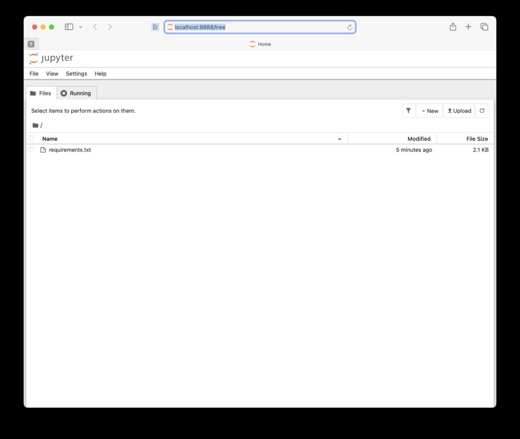
The code to perform PCA using Scikit-learn on Iris is run on Jupyter Notebook, start it below:
jupyter notebook
This launches a browser with the local Jupyter notebook as the web page.
5.4 Import Libraries and Load the Iris Dataset
Here we set up a foundation for preprocessing running PCA using Scikit-Learn.
We import our libraries.
import numpy as np
import pandas as pd
import matplotlib.pyplot as plt
import seaborn as sns

from sklearn.datasets import load_iris
from sklearn.preprocessing import StandardScaler
from sklearn.decomposition import PCA
from sklearn.model_selection import train_test_split
from sklearn.linear_model import LogisticRegression
from sklearn.metrics import accuracy_score
Next, we load the dataset.
# Load the iris dataset
iris = load_iris()
X = iris.data
y = iris.target
feature_names = iris.feature_names
target_names = iris.target_names

# Convert to DataFrame for readability
df = pd.DataFrame(X, columns=feature_names)
df['target'] = y
We also do a sanity check, but that is perfectly optional with you.
print(df.head())
print(df['target'].value_counts())
5.5 Standardize the Features
For PCA using Scikit-learn to work properly, we must standardize the features so they have zero mean and unit variance.
# Standardize the features
scaler = StandardScaler()
X_scaled = scaler.fit_transform(X)
5.6 Apply PCA using Scikit-Learn from sklearn.decomposition
Finally, we are ready to apply PCA to our dataset using the following code.
# Apply PCA and keep all components
pca = PCA()
X_pca = pca.fit_transform(X_scaled)
5.7 Plot Explained Variance Ratio
Now that we have applied PCA using Scikit to our dataset, we would like to visualize our results to understand how PCA works.
# Plot explained variance ratio
plt.figure(figsize=(8, 4))
plt.plot(np.cumsum(pca.explained_variance_ratio_), marker='o')
plt.title('Cumulative Explained Variance by PCA Components')
plt.xlabel('Number of Components')
plt.ylabel('Cumulative Explained Variance')
plt.grid(True)
plt.tight_layout()
plt.show()
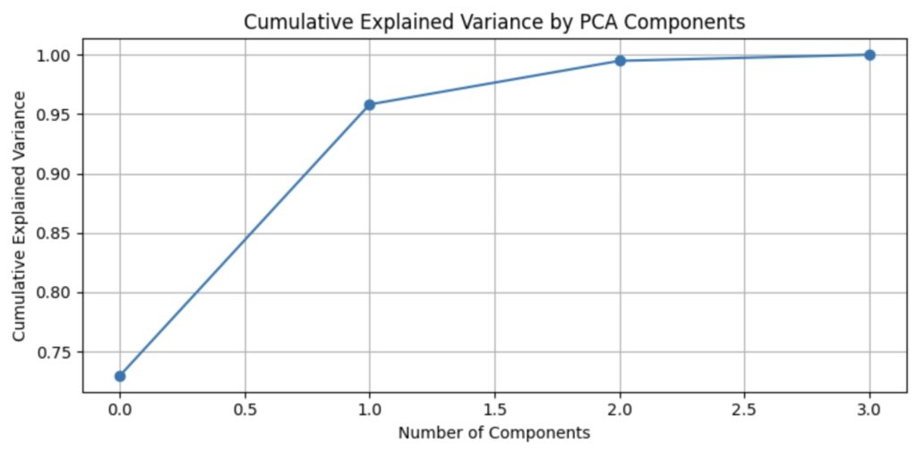
The plot of cumulative explained variance by PCA components is shown below.
5.8 2D Scatter Plot – Visualize First Two Principal Components
From the plot above, we see that two components explain the most significant portion of the variance. We now want to see how they affect the datapoints through a scatter plot using the following code.
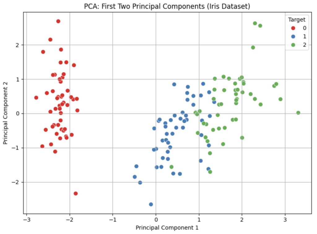
# Create a DataFrame for the first two principal components
pca_df = pd.DataFrame(X_pca[:, :2], columns=['PC1', 'PC2'])
pca_df['target'] = y

# Plot the 2D PCA result
plt.figure(figsize=(8, 6))
sns.scatterplot(data=pca_df, x='PC1', y='PC2', hue='target', palette='Set1', s=60)
plt.title('PCA: First Two Principal Components (Iris Dataset)')
plt.xlabel('Principal Component 1')
plt.ylabel('Principal Component 2')
plt.legend(title='Target')
plt.grid(True)
plt.tight_layout()
plt.show()
This yields the scatter plot below where we can easily discern the three major clusters. We note that only clusters two and three have some overlap.
5.9 Compare Classifier Accuracy Before and After PCA using Scikit-Learn
We now want to confirm that PCA using Scikit-Learn will preserve accuracy in our data. We measure our data’s accuracy before applying PCA and then measure after applying PCA.
5.9.1 Accuracy Before PCA
We run the following code to obtain the accuracy of the data. We applied PCA to it.
# Split the original (unscaled) data
X_train_orig, X_test_orig, y_train, y_test = train_test_split(X, y, test_size=0.3, random_state=42)

# Train Logistic Regression on original data
clf_orig = LogisticRegression(max_iter=1000)
clf_orig.fit(X_train_orig, y_train)
y_pred_orig = clf_orig.predict(X_test_orig)
accuracy_orig = accuracy_score(y_test, y_pred_orig)

print("Accuracy without PCA:", round(accuracy_orig, 3))
This provided the following result.
Accuracy without PCA: 1.0
5.9.2 Accuracy After PCA
We run the following code to obtain the accuracy of the data after we applied PCA to it. This time, we train the logical regression model on the PCA data and compare its predicted values to the original values.
# Split PCA-transformed data
X_train_pca, X_test_pca, _, _ = train_test_split(X_pca, y, test_size=0.3, random_state=42)

# Train Logistic Regression on PCA-transformed data
clf_pca = LogisticRegression(max_iter=1000)
clf_pca.fit(X_train_pca, y_train)
y_pred_pca = clf_pca.predict(X_test_pca)
accuracy_pca = accuracy_score(y_test, y_pred_pca)

print("Accuracy with PCA:", round(accuracy_pca, 3))
We actually got the result below, where no accuracy was lost!
Accuracy with PCA: 1.0
5.9.3 Comments on the Comparison
These accuracies are shown in the following chart.
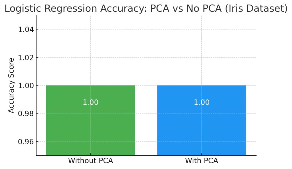
PCA maintained perfect accuracy on the Iris dataset, demonstrating that dimensionality reduction can simplify the input space without compromising model performance when the principal components capture the core variance.
6. Best Practices for PCA in Scikit-Learn and Common Pitfalls to Avoid
PCA using Scikit-Learn is a powerful preprocessing tool, especially for classification and clustering models. However, it is important to use it properly, otherwise it can cause models to yield inaccurate results.
The first rule when using PCA is to always standardize your dataset before applying PCA to it. Standardizing your dataset will ensure that each feature contributes equally to the PCA. Failure to standardize your dataset will have features with larger scales dominating the principal components. This is because PCA assumes all input variables are on the same scale when computing covariances.
It is also important to check whether a dimension is really redundant before removing it. Reducing too many dimensions can discard critical information that is detrimental to model performance. Always check the explained variance to make sure we retain all the components that capture meaningful information.
A major limitation of PCA is that it always assumes linearity and may not adequately capture the dataset’s non-linear relationships. When patterns do go beyond linear variances, then use nonlinear methods like t-SNE or UMAP.
It is always important to remember that using PCA never guarantees better accuracy. Therefore, we must always test its impact on our models. It is important to perform cross-validation to ensure that PCA enhances rather than damages performance.
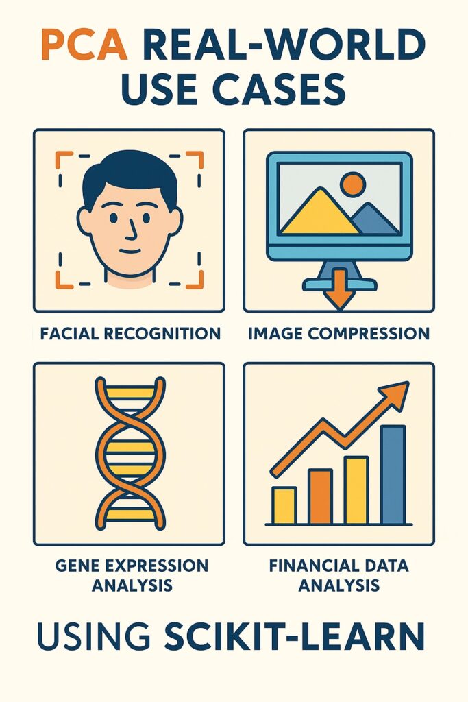
7. Use Cases in Real-World Applications with PCA in Scikit-Learn
It is worthwhile considering some real-world examples where PCA in Scikit-Learn is useful. A common use is for facial recognition, which has many tangible applications. Here we derive eigenfaces that use PCA to reduce facial images into key components for efficient recognition. These eigenfaces capture the most significant variance across faces, which enables dimensionality reduction. Facial recognition systems can compare new faces against the stored Eigenface projection to classify these new faces.
Another important use for PCA using Scikit-Learn is image compression in order to reduce the data stored for each image. Here, PCA compresses images by keeping only the principal components that capture most of the variance. Hence, we reduce storage needs while preserving the original image’s key visual features.
Gene expression data is an important category for dimensionality reduction, given the vast amount of data we need to process. Here, we can use PCA to simplify gene expression data by reducing thousands of gene variables into key patterns. It achieves this by identifying groups of genes with correlated behavior across different samples or conditions.
Financial data analysis is another key application that utilizes PCA with Scikit-Learn. This is because it reduces correlated financial indicators into independent components for clearer trend analysis. Additionally, it assists by uncovering hidden market structure and allows for more stable predictive modeling.
8. Conclusion and Next Steps
PCA using Scikit-Learn is a valuable tool for dataset preprocessing for ML models that perform classification and clustering. Its main use is simplifying complex data and removing redundancies that ML models do not need to learn from scratch. It also enables understanding through principal components that we can easily visualize.
The Iris dataset can also effectively demonstrate the benefit of PCA simplification with its relatively small size and small feature space. However, experimenting with other datasets will provide a greater appreciation of PCA’s value in uncovering the data’s underlying structure.
PCA’s real value is when it is used in conjunction with other preprocessing activities. We should first apply feature selection to the dataset, allowing PCA to work with only the relevant features. This improves its efficiency and reduces the possibility of any noise affecting its accuracy.
PCA can only uncover linear structures but cannot discover non-linear patterns or data clustering. t-SNE can further process PCA’s output to capture non-linear relationships. In turn, clustering can identify patterns or groups from the t-SNE output that are not obvious in the original data space.
You now have the means to begin your own PCA journey with the code in this article. Please work through this and embark on your own discovery of PCA with Scikit-Learn.
10. Foundational References
Pearson, K. (1901). On lines and planes of closest fit to systems of points in space.
Philosophical Magazine, 2(11), 559–572.
— The original PCA paper introducing the method.
Jolliffe, I. T., & Cadima, J. (2016). Principal component analysis: A review and recent developments.
Philosophical Transactions of the Royal Society A, 374(2065).
— Comprehensive modern review on PCA, including theory and extensions.
11. Official Documentation on PCA using Scikit-Learn
PCA Documentation
— API documentation for PCA in Scikit-learn, with examples.
PCA User Guide – Decomposition: PCA
— Detailed guide with explanations, math, and practical guidance.
12. Further Reading in PCA using Scikit-Learn
“Hands-On Machine Learning with Scikit-Learn, Keras, and TensorFlow” – Aurélien Géron
ISBN: 9781098125974
— Chapter on unsupervised learning covers PCA with practical examples.
“Python Machine Learning” – Sebastian Raschka & Vahid Mirjalili
ISBN: 9781800567701
— Explains PCA thoroughly with Scikit-learn implementations.