1. Introduction to How to Deal With Imbalanced Data in Classification
Here we will show how to deal with imbalanced data in classification that often occurs in the real world. Some everyday examples of classifying imbalanced data include fraud detection, health, and rare event (black swan) event prediction. We define imbalanced data in classification as datasets where one class significantly outnumbers the other classes. This often leads to biased model performance.
Accordingly, we will consider the above examples in relation to imbalanced data in classification. Fraud detection is a notable example of imbalanced data, where fraudulent transactions are rare in comparison to legitimate ones. Similarly, imbalanced data can have severe consequences for healthcare when diagnosing rare conditions. Chiefly, positive cases are significantly fewer than negative ones. Furthermore, imbalanced data also affects rare event prediction since these events seldom occur. Examples of the events that seldom occur include equipment failure or security breaches.
Therefore, learning how to deal with imbalanced data in classification is critical for machine learning. Firstly, when we train machine learning models on imbalanced data. Such machine learning models often favor the majority and reduce accuracy for rare but essential outcomes. Consequently, they provide misleading metrics, such as high overall accuracy but poor recall for minority classes. Therefore, when we properly address imbalances, we improve model fairness, reliability, and real-world decision-making.
AWS provides tools like Sagemaker and Glue that support Exploratory Data Analysis (EDA) workflows. These workflows are especially important in identifying and correcting class imbalance early in the ML pipelines.
2. Signs of Imbalanced Data
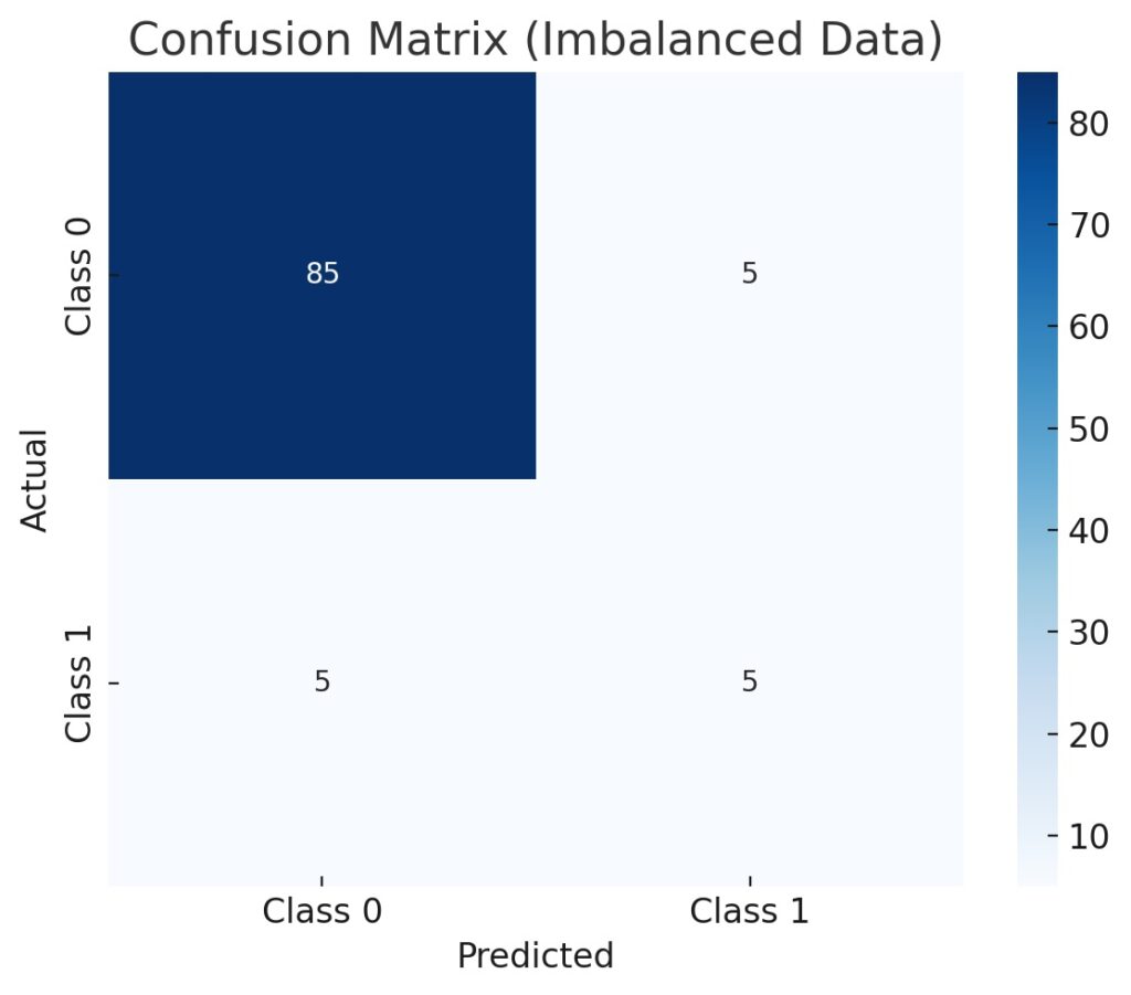
Whenever considering how to deal with imbalanced data in classification, we need to look for signs of imbalanced data. Therefore, we need to be able to detect imbalances in datasets. Firstly, we need to calculate the frequency of each class to check for any skewed distributions. Typically, we do this by plotting a bar chart of class counts to visualize any imbalances. Additionally, we obtain a quick class summary by using the value_counts() function in Pandas. Subsequently, we should compute the imbalance ratio by dividing the majority class counts by the minority class counts. Additionally, we should also inspect confusion matrices from a baseline model to detect any performance gaps. Specifically, we need to compare accuracy to recall and precision to spot hidden class bias.
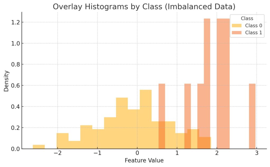
There are several class distribution examples that show how to spot imbalanced data for classification. Firstly, Seaborn’s library provides the countplot() function that generates a bar plot clearly showing class imbalance at a glance. Furthermore, we can use Matplotlib to plot custom class distributions with labels for exact counts. Also, pie charts are handy for providing quick visualizations of class properties. Another example is that we can plot separate histograms for each class to compare feature distributions. Additionally, we can overlay these histograms with KDE plots by class to detect subtle differences in data shape. Finally, we can construct fast distribution charts using Pandas’ plot(kind=’bar’) on value_counts().
Accuracy
We need to understand how to deal with imbalanced data in classification since accuracy suffers from imbalanced data. Specifically, imbalanced data makes accuracy appear high even when the model is ignoring the minority class. Subsequently, it masks poor performance on rare but important outcomes. Rather, high accuracy may reflect class imbalances, but not true predictive power. Furthermore, accuracy fails to capture false negatives and false positives effectively. Therefore, modeling with imbalanced data will consider data precision, recall, and F1-score, which are also associated with the confusion matrix.
3. EDA Techniques to Deal With Imbalanced Data in Classification
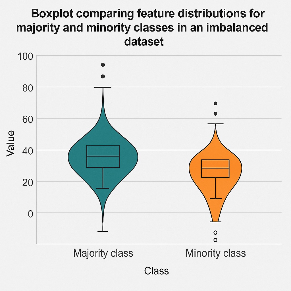
EDA provides some useful techniques on how to deal with imbalanced data in classification. Specifically, the secret weapon in understanding and analyzing data is visualization using plots like histograms, boxplots, and violin plots. Histograms show how feature values are distributed across different classes. They especially help in revealing skewness, gaps, or overlaps in class distributions. Boxplots are another valuable visualization tool that summarizes median, quartiles, and outliers for each class. Accordingly, they make it easy to spot class-specific variability or extreme values. Violin plots also help reveal insights by combining boxplot statistics with distribution shapes. They subsequently highlight subtle class differences that histograms may miss.
Feature Relationships Based on Class Membership
Aside from these plots, another set of valuable techniques is analyzing how features relate based on their class membership. Basically, grouping data by class can help reveal how features behave differently across different categories. This can uncover patterns that may be obscured when examining the overall dataset and point to imbalances between categories. Another characteristic of features we are interested in is how they cluster or overlap, which can show imbalance. Therefore, we use scatter plots to help reveal these. We also want to know hidden dependencies that correlation matrices segmented by class help bring to light. These hidden dependencies can also show how imbalances may arise. We further reveal these through inspecting feature interactions, which show different effects depending on the class.
Furthermore, pair plots are another helpful tool in our arsenal, allowing multi-feature comparison across classes. These help expose interactions and joint patterns between features that are not apparent when analyzing them individually. These interactions and joint patterns also help us deal with imbalanced data in classification. Additionally, summary statistics remain crucial in revealing differences in mean and variance. For more hands-on guidance on visual techniques like histograms, boxplots, and pair plots, check out our data visualization guide in Python. These mean and variance differences across classes reveal whether a feature contributes to the imbalance or helps separate the classes.
Python Tools
Correspondingly, specific Python libraries support these plots and visualizations, including Pandas, Seaborn, and Matplotlib.
4. Resampling Strategies that Deal With Imbalanced Data in Classification
Although we have considered finding imbalanced data in classification, we now want to explore how to deal with it. Basically, the most common strategies are resampling either the majority class or the minority class, or both. Therefore, we will now survey these strategies.
4.1 Undersampling
This is connected with reducing the size of the majority class by randomly undersampling it. Therefore, this helps balance class distribution by removing excess majority samples and is simple and easy to implement. Furthermore, reducing the overall number of samples can help speed up training with a reduced dataset size. However, data scientists also need to consider the risk of discarding useful information from the majority class. Another consequence is that undersampling can lead to underfitting whenever too much data is removed. Therefore, this technique is most effective whenever the majority class has redundant or highly similar samples.
Nevertheless, this is often used as a baseline before exploring more advanced techniques that deal with imbalanced data in classification. However, it works best when the dataset is large enough that reducing the majority class will not harm overall learning. Moreover, we can combine this with cross-validation to minimize any risk of performance loss.
4.2 Oversampling
Conversely, instead of undersampling the majority classes, we can oversample the minority classes. This is another approach to deal with imbalanced data in classification. Here, we often duplicate existing minority class examples when oversampling, thereby increasing the minority class’s representation. Therefore, the main advantage is that we balance class distribution without losing data. Another benefit is that duplicated examples provide the model with more exposure to rare cases.
However, we now risk misleading the model by repeatedly exposing it to the same examples. This can also cause the model to memorize rather than to generalize. Another issue is that overfitting can lead to poor performance on any data that was never used to train the model. Also, minority classes that are very small can increase the risk of overfitting. This leads to validation metrics looking good during training but failing in production. However, combining oversampling with cross-validation can help detect and reduce overfitting.
4.3 SMOTE and Variants
Notably, both oversampling and undersampling techniques have their advantages and disadvantages. Therefore, we now consider various synthetic sampling techniques that help deal with imbalanced data in classification. These synthetic sampling techniques generate new samples for the minority class based on existing data. Particularly, SMOTE techniques generate samples by interpolating between real examples. Therefore, they help models learn decision boundaries more effectively. Also, unlike simple duplication, they reduce the risk of overfitting.
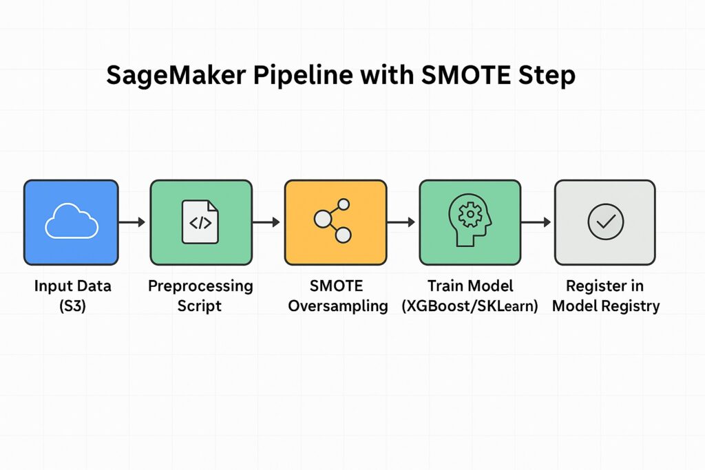
Additionally, combining these synthetic oversampling techniques with cross-validation helps to ensure robust model evaluation. Cross-validation also helps detect whenever synthetic samples lead to data leakage of the validation set, unintentionally influencing the model during training. Therefore, pipelines should ensure that oversampling is only applied to training folds and not to test sets. Also, we can find support for SMOTE and its variants in the imbalance-learn Python library. We can also customize SageMaker Processing scripts to apply SMOTE during data preparation. Finally, using tools like Pipeline from scikit-learn or SageMaker Pipelines will keep preprocessing repeatable and scalable.
5. Modeling to Deal with Imbalanced Data in Classification
We can also build classification models that accurately learn from uneven class distributions without introducing biases toward the majority class.
5.1 Precision, Recall, F1, and AUC
Accuracy is insufficient when we have to deal with imbalanced data in classification for machine learning models. We need other metrics.
Precision measures how many predicted positives are actually correct. Therefore, low precision indicates the model labels many majority class samples as minority class, resulting in false alarms.
Conversely, recall indicates how well the model captures true positives from all actual positives. Therefore, low recall indicates the model is failing to identify many actual minority class cases. Hence, it is overlooking many important but rare events, such as fraud or disease.
We should also combine precision and recall into a single metric, F1. Whenever the F1 score is low, then either precision or recall, or both, are weak. This results in poor detection of the minority class. Conversely, when the F1 score is high, then the model is effectively identifying the minority class without excessive false alarms.
Finally, we have the Area Under the Curve (AUC), which summarizes the model’s ability to distinguish between classes. Like F1, this metric also indicates good performance on both minority and majority classes.
5.2 Tree-Based Models
Additionally, tree-based models often perform well on imbalanced data, with popular implementations including Random Forest and XGBoost. Chiefly, they can handle non-linear relationships and can adjust to class imbalance using built-in parameters.
5.3 Scikit-learn models
The scikit-learn library models can automatically adjust the weights of each class inversely to their frequencies by setting class_weight=’balanced’. Subsequently, the model can pay more attention to the minority class without needing to resample the data manually.
5.4 Threshold Tuning to Deal with Imbalanced Data in Classification
Another approach to address imbalanced data in classification is to tune the threshold after training a classification model. We can select the decision boundary based on our application goals, which are either minimizing false negatives or false positives.
6. AWS Tools to Handle Imbalanced Data in Classification
Specifically, AWS provides several tools that are well-suited for handling imbalanced data in classification.
SageMaker particularly provides built-in support for class weights with XGBoost, allowing us to set scale_pos_weight to handle class imbalance. It also provides the SageMaker Estimator API, allowing us to pass weights directly in custom training scripts. SageMake is also integrated with scikit-learn, which supports class_weight=’balanced’ during training.
Additionally, SageMaker Processing lets us apply SMOTE or undersampling during preprocessing at scale. It also allows us to write custom scripts that balance data before training using Pandas and imbalanced-learn. These processing jobs integrate seamlessly into SageMaker Pipelines for automated data balancing and processing.
Other services lend themselves to helping to address imbalanced data with classification. Specifically, AWS Glue enables us to clean, transform, and prepare large datasets for modeling. Additionally, Glue Jobs supports PySpark scripts, which enable us to perform scalable resampling and feature engineering. Correspondingly, we can use AWS Athena to query our preprocessed data to verify class distributions and data quality. Therefore, we can combine Glue and Athena for a repeatable, serverless data validation workflow. For a deeper dive into scalable data cleaning and preparation techniques on AWS, see our guide on ML data preprocessing.
We also have SageMaker Notebooks available for quick experimentation and visual EDA. Subsequently, we can switch to SageMaker Pipelines for repeatable, automated training workflows. Using Pipelines reduces manual steps and helps prevent data leakage in production.
7. Best Practices and Common Pitfalls
Whenever balancing data for classification, there are several best practices and pitfalls to avoid. Notably, a common pitfall is that oversampling without validation can lead to overfitting. Also, repeated exposure to identical samples can degrade model generalization. Consequently, it is vital to combine oversampling with cross-validation to check real-world performance.
Following on from this, we should always test model performance on data that is not used in resampling. This is because untouched validation sets help prevent misleading performance estimates. Therefore, they help detect overfitting and data leakage during the evaluation process.
Data leakage is where training data leaks into validation data, inflating performance metrics and making evaluation misleading. Therefore, we should ensure that resampling only applies to training data and not validation data. Subsequently, we should track data flow carefully in pipelines to avoid contamination.
Meanwhile, we often need to make trade-offs between precision and recall and need to align this with business outcomes. Subsequently, we need to use metrics that reflect the true cost of false positives and false negatives. Specifically in healthcare and fraud, we should prioritize recall where missing cases are critical. However, there are other applications where we want to avoid false alarms; hence, we prioritize precision.
8. Conclusion
Imbalanced data in classification systems poses several challenges, and there are strategies for both data preprocessing and model refinement. Firstly, detection is important to understand that high accuracy is potentially misleading. Next, it is valuable to visualize any imbalances to gain an intuitive understanding and better address them. Subsequently, we can apply various resampling strategies before training our model. Additionally, we can select training algorithms and parameters that also address imbalances and allow us to make any necessary trade-offs. Finally, it is also important to monitor performance and use validation data that is free from any resampling.
AWS provides a suite of tools that allow us to incorporate these strategies into any ML workflow and at scale.
9. Further Reading
“Imbalanced Learning: Foundations, Algorithms, and Applications” By Haibo He and Yunqian Ma
This is the most comprehensive reference book on the subject, widely cited in academia and industry.
“Hands-On Machine Learning with Scikit-Learn, Keras, and TensorFlow” By Aurélien Géron
Includes practical sections on class imbalance handling using real-world datasets and scikit-learn.
“Python Machine Learning” By Sebastian Raschka and Vahid Mirjalili
Covers precision, recall, F1-score, and techniques like SMOTE with strong applied examples.
“Machine Learning with Python Cookbook” By Chris Albon
Offers recipes for handling imbalanced data using imbalanced-learn, along with model evaluation strategies.
“Applied Predictive Modeling” By Max Kuhn and Kjell Johnson
While broader in scope, it has in-depth examples of handling imbalanced data for classification problems.
“Learning from Imbalanced Data Sets” by Fernández et al.
Provides a comprehensive overview of techniques, challenges, and algorithms for effectively handling class imbalance in machine learning across diverse application domains.
Affiliate Disclosure: This post contains affiliate links. If you click through and make a purchase, we may earn a small commission at no extra cost to you. As an Amazon Associate, AI Cloud Data Pulse earns from qualifying purchases. We only recommend products we believe add real value to our readers.
10. References
He, H., & Garcia, E. A. (2009). Learning from imbalanced data.
IEEE Transactions on Knowledge and Data Engineering, 21(9), 1263–1284.
Chawla, N. V., Bowyer, K. W., Hall, L. O., & Kegelmeyer, W. P. (2002). SMOTE: Synthetic Minority Over-sampling Technique.
Journal of Artificial Intelligence Research, 16, 321–357.
Lemaître, G., Nogueira, F., & Aridas, C. K. (2017). Imbalanced-learn: A Python Toolbox to Tackle the Curse of Imbalanced Datasets in Machine Learning.
Journal of Machine Learning Research, 18(17), 1–5.