Train Model with TensorFlow for Beginners

Introduction to Training TensorFlow Models

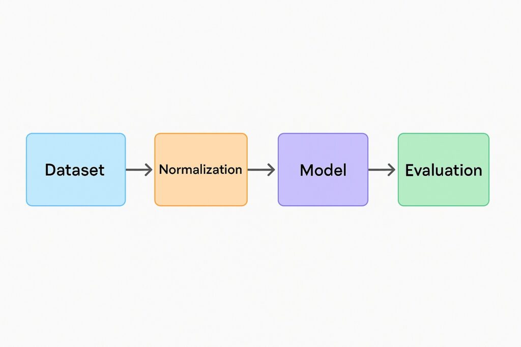
This is a step-by-step TensorFlow tutorial for beginners, where we will train a machine learning model. We will use structured datasets, perform preprocessing with normalization, define a Sequential API network, and save the trained model for future use.

Machine learning differs from traditional computer programming, where the algorithm learns from data instead of executing an instruction set. What is amazing about this? The algorithm learns by itself to recognize patterns based on the training data. It achieves this by adjusting the model’s parameters over time to improve predictions and minimize errors. Training models using the TensorFlow framework is a popular choice for many ML engineers and organizations. Its framework can build and train models on CPUs, GPUs, or TPUs in a scalable way. TensorFlow has a rich ecosystem and a large, active user community, making it appealing both to beginners and seasoned practitioners.

This guide introduces the beginner to training models with TensorFlow by breaking down the training process into clear, manageable steps. It explains each step with simple examples so beginners can follow along without feeling lost. This guide will teach readers how to set up TensorFlow in their development environment. They will also get familiar with how to train a model using structured datasets and monitor progress. Next, this guide will lead them to evaluate model performance using test data. Last, the reader will learn how to save the trained TensorFlow model for future use or development.

We have tried to target this to a wide range of beginners, including novices, existing ML hobbyists, and of course, students. Now it is time for them to get their hands dirty using TensorFlow to train models.

Model Training for Newbies

What does model training actually mean? Well, it is how we teach a machine learning algorithm to make accurate predictions from data. We have the algorithm comparing its predictions to the correct answers, and it continually makes internal adjustments. When its predictions are close enough to the expected answer, we expose it to new data that it hasn’t seen. Therefore, it can make predictions for us.

Training data consists of the examples that a model needs to learn to make reliable predictions, even with TensorFlow. Given its importance, we need to ensure it is of high quality in several ways. Training data must accurately represent the problem space, ensuring the model performs well in real scenarios. We must remove biases so that the model does not produce outputs that are inaccurate or unreliable.

How does a model make internal adjustments, you may say? Well, it is continually changing its parameters like weights and biases upon each comparison of its prediction with the correct data. It uses optimization algorithms to provide the changes that it needs to fine-tune these parameters for minimizing the differences between predicted and actual results.

Now, why would we use TensorFlow for training a model? Well, it provides a flexible set of tools that make building and training models efficient across a range of hardware. It also provides scalability where beginners and experts can tackle projects of any size. However, its active community support can help all members address any blockers.

Setting Up TensorFlow

This is a hands-on approach to training a model using TensorFlow, and we will show how to set up TensorFlow. This demonstration is done on a MacBook Pro with M4 Ultra Chip, 48 GB RAM, and 1 TB SSD. The version of Python installed on the MacBook Pro is Python 3.12.3, and the version of pip installed is pip 24.0.

Install TensorFlow

We created a directory to do our work, and will now create a virtual environment under that directory using the following command.

python3 -m venv venv

Once we created our virtual environment, we activated it using:

source venv/bin/activate

Once activated, the prompt became:

(venv) your-macbook directory %

Typically, we would use the following commands to install TensorFlow within our environment:

pip install --upgrade pip

pip install tensorflow

However, if you are using Apple Silicon, do as we did and use the following commands to install TensorFlow:

python -m pip install --upgrade pip setuptools wheel

pip install tensorflow-macos

pip install tensorflow-metal

Verify TensorFlow Installation for Training Models

Since we are doing this on a MacBook Pro M4, we ran the following commands to verify prerequisites:

pip show tensorflow-macos tensorflow-metal

python -c "import platform; print(platform.machine())" # should print: arm64

We will also run all other commands within the Python shell and show how to verify when not using Apple with Apple Silicon.

To start the Python shell, we typed the following in our virtual environment:

python

Non-Apple Silicon With GPU

When not on Apple Silicon and you want to verify that the GPU is visible to the system, then type:

nvidia-smi

Now, verify that TensorFlow can see the GPU which is used to train our model

import tensorflow as tf
print("TensorFlow version:", tf.__version__)
print("GPUs:", tf.config.list_physical_devices("GPU"))

Expected: At least one GPU in the list and “Built with CUDA: True”.

Run the following to see the GPU at work and confirm TensorFlow is using the NVIDIA GPU properly

with tf.device("/GPU:0"):
    a = tf.random.normal([1024, 1024])
    b = tf.random.normal([1024, 1024])
    c = tf.matmul(a, b)
    print("OK:", c.shape)

Non-Apple Silicon Without GPU

Now, verify that TensorFlow can see the GPU that is used to train our model with

import tensorflow as tf
print("TensorFlow version:", tf.__version__)
print("GPUs:", tf.config.list_physical_devices("GPU"))
print("Built with CUDA:", tf.test.is_built_with_cuda())

Apple Silicon

Here, verify the Apple Silicon architecture

python -c "import platform; print(platform.machine())"   # should print: arm64

Next, we run the GPU computation test

import tensorflow as tf

with tf.device("/GPU:0"):
    a = tf.random.normal([1024, 1024])
    b = tf.random.normal([1024, 1024])
    c = tf.matmul(a, b)
    print("OK:", c.shape)

Preparing Your Dataset

Dataset preparation is a critical step in the ML workflow for training our model with TensorFlow, and we will show a practical example below. We selected California Housing as a sample to demonstrate the necessity of dataset preparation since it needs several preprocessing steps.

Workflow diagram showing dataset, normalization, model, and evaluation steps in TensorFlow

Loading datasets

We will set up the URLs to download our California Housing data and the features for our dataset. Again, we enter the Python shell and run the following code:

import tensorflow as tf

TRAIN_URL = "https://download.mlcc.google.com/mledu-datasets/california_housing_train.csv"
TEST_URL  = "https://download.mlcc.google.com/mledu-datasets/california_housing_test.csv"

FEATURES = [
    "longitude", "latitude", "housing_median_age", "total_rooms",
    "total_bedrooms", "population", "households", "median_income"
]
LABEL = "median_house_value"
BATCH_SIZE = 64
AUTOTUNE = tf.data.AUTOTUNE

Once we have set our URLs and our schemas, we download the CSV files from the internet and upload them to TensorFlow datasets.

train_path = tf.keras.utils.get_file("california_housing_train.csv", TRAIN_URL)
test_path  = tf.keras.utils.get_file("california_housing_test.csv", TEST_URL)

ds_train = tf.data.experimental.make_csv_dataset(
    file_pattern=[train_path],
    batch_size=BATCH_SIZE,
    label_name=LABEL,
    num_epochs=1,          # set None for infinite epochs
    shuffle=True,
    header=True
)

ds_test = tf.data.experimental.make_csv_dataset(
    file_pattern=[test_path],
    batch_size=BATCH_SIZE,
    label_name=LABEL,
    num_epochs=1,
    shuffle=False,
    header=True
)

Preprocessing

We also want to make our data easier for a machine learning model to load and ingest. Loading our data above, we have a tensor for each feature shown below.

 { "median_income": tensor([ ... ]), "housing_median_age": tensor([ ... ]), ... }

This is easy for a human to read, but not efficient for a model. Therefore, it expects the tensors combined into one single dense tensor as below.

 [[v11, v12, v13, ...], [v21, v22, v23, ...], ...]

The following code packs our tensors into a single, large tensor for machine learning.

def pack(features, label):
    # Stack selected numeric columns into a [batch, num_features] tensor
    cols = [tf.cast(features[name], tf.float32) for name in FEATURES]
    x = tf.stack(cols, axis=-1)   # shape: [batch, 8]
    y = tf.cast(label, tf.float32)
    return x, y

ds_train = ds_train.map(pack, num_parallel_calls=AUTOTUNE)
ds_test  = ds_test.map(pack,  num_parallel_calls=AUTOTUNE)

We selected California Housing because its features vary widely with (medium_income vs total_rooms vs latitude/longitude). This is a problem for ML models, and normalizing these values so they have similar ranges prevents any one feature from dominating. This helps the optimizer algorithm and enhances training speed. The following code performs this normalization.

norm = tf.keras.layers.Normalization(axis=-1)
# Adapt expects only features; strip labels
norm.adapt(ds_train.map(lambda x, y: x))

def apply_norm(x, y):
    return norm(x), y

ds_train = ds_train.map(apply_norm, num_parallel_calls=AUTOTUNE).prefetch(AUTOTUNE)
ds_test  = ds_test.map(apply_norm,  num_parallel_calls=AUTOTUNE).prefetch(AUTOTUNE)

Defining the Model for Training with TensorFlow

Models for training with TensorFlow are neural networks trained with an optimizer algorithm. Therefore, our next step is to define the structure of our neural network. We select the Sequential API, which is a simple stack of layers, making the model purely linear in flow.

Sequential API example

Since the Sequential API is a simple model, there are only a handful of parameters that we need to set up. The code for our model is shown below:

model = tf.keras.Sequential([
    tf.keras.Input(shape=(len(FEATURES),)),  # shape matches your feature vector
    norm,                                    # Normalization as first layer
    tf.keras.layers.Dense(32, activation="relu"),
    tf.keras.layers.Dense(16, activation="relu"),
    tf.keras.layers.Dense(1)                 # Regression output
])

Given that it is a stack of layers, we define the number of layers for our model for training with TensorFlow. The first layer is the input layer, and this is where we also do our normalization as discussed earlier. The subsequent two layers are our neural layers, whose weights we train using an optimization algorithm. The final layer is a single neuron representing our output function, which is the median housing price.

Using two middle layers is a balanced default for small-to-medium tabular datasets like the California Housing dataset. Having just one middle layer makes the model too shallow. While it can still learn non-linear relationships, it may struggle to capture complex feature interactions in high-dimensional data. On the other side of the coin, we implemented only two layers because of the limited samples, which can result in overfitting.

We adopted a progressive narrow design by having half the number of neurons in the second middle layer. This works well for tabular data of this size, and we have 32 and 16 neurons, respectively, which is a good starting point.

Finally, the ReLU (Rectified Linear Unit) was selected as the activation function. Experience has shown it to be the most effective activation function.

Compiling and Training the Model with TensorFlow

We are finally ready to compile and train our model with the TensorFlow framework.

Compiling the Model

Previously, our model definition established the blueprint for our model, but we now want to wire in our rules for training. We refer to this activity as compiling the model and invoke TensorFlow’s model.compile(…) function to set up our training rules. The compilation code is shown below:

model.compile(
    optimizer=tf.keras.optimizers.Adam(learning_rate=0.001),
    loss="mse",          # regression loss
    metrics=["mae"]      # monitor mean absolute error
)

The three parameters specify the optimization algorithm, the loss function, and the metrics to monitor.

The model uses the optimization algorithm to adjust the weights during training, and there are several types. The simplest is stochastic gradient descent. However, linear models typically use the adaptive learning rate (adam), which is the one that we are using.

The loss function measures the error between the model output and the actual value that the model is trying to attain. For regression, the loss function is typically the mean squared error or the mean absolute error. In the case of classification, the loss function is generally categorical_crossentropy or binary_crossentropy.

Metrics are optional, and the engineer uses these to monitor performance and appear in the training logs.

Whenever the compile function is invoked, TensorFlow wires up the computational graph so the model is ready for training.

Training the Model with TensorFlow

To actually train the model, we invoke the model.fit() as shown below.

history = model.fit(
    ds_train.prefetch(tf.data.AUTOTUNE),
    validation_data=ds_test.prefetch(tf.data.AUTOTUNE),
    epochs=5
)

We fetch both the training and test data and specify the number of epochs. Epochs specify the number of times the entire training set is run through the model during training. Here, we want to tune since too few epochs result in underfitting, while too many result in overfitting.

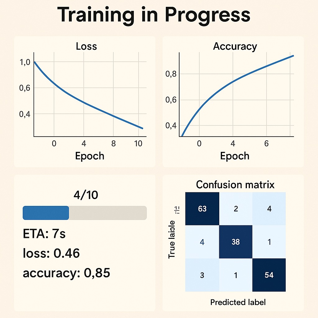
When executing, the model shows its progress, and TensorBoard is available to monitor training.

Evaluating and Saving the Model Trained with TensorFlow

Once we have trained our model with TensorFlow, we turn to evaluating it using the model.evaluate () function on the test data. The code is shown below:


loss, mae = model.evaluate(ds_test)
print(f"Test MAE: {mae:.4f}")

We had a relatively high MSE of 200k. Therefore, we retrained with 200 epochs and implemented tf.keras.callbacks.EarlyStopping() when the loss function stopped improving. We also used the Huber function to minimize outliers. The updated training code is shown below.


import tensorflow as tf

model.compile(
    optimizer=tf.keras.optimizers.Adam(learning_rate=0.001),
    loss=tf.keras.losses.Huber(delta=1.0),   # or try 2.0 / 5.0
    metrics=["mae"]
)

early_stop = tf.keras.callbacks.EarlyStopping(
    monitor="val_mae", patience=10, mode="min", restore_best_weights=True
)

history = model.fit(
    ds_train.prefetch(tf.data.AUTOTUNE),
    validation_data=ds_test.prefetch(tf.data.AUTOTUNE),
    epochs=200,
    callbacks=[early_stop],
    verbose=1
)

loss, mae = model.evaluate(ds_test.prefetch(tf.data.AUTOTUNE))
print(f"Test MAE: {mae:.2f}")

This reduced the MSE to 50K, although still high, and further alterations around layer density, outliers, and logarithmic functions are necessary. Our purpose is to demonstrate training a model with TensorFlow, and we will explore improving model performance in a future article.

Training process snapshot showing loss and MAE curves during TensorFlow model fitting

We more than likely want to continue working with our model to improve its performance. Also, when its performance is satisfactory, then we want to use it as an inference engine. Therefore, we use model.save() for further training and use for inference. We implemented the code below to save our model.


# Save in the recommended Keras format
model.save("california_housing_model.keras")

TensorFlow code script flow from data loading to model saving

When we want reload our model for further training or inference we invoke the tf.keras.models.load_model() method. This is shown in the code below for our demonstration.


# Load back
restored_model = tf.keras.models.load_model("california_housing_model.keras")

Best Practices for Training Models in TensorFlow

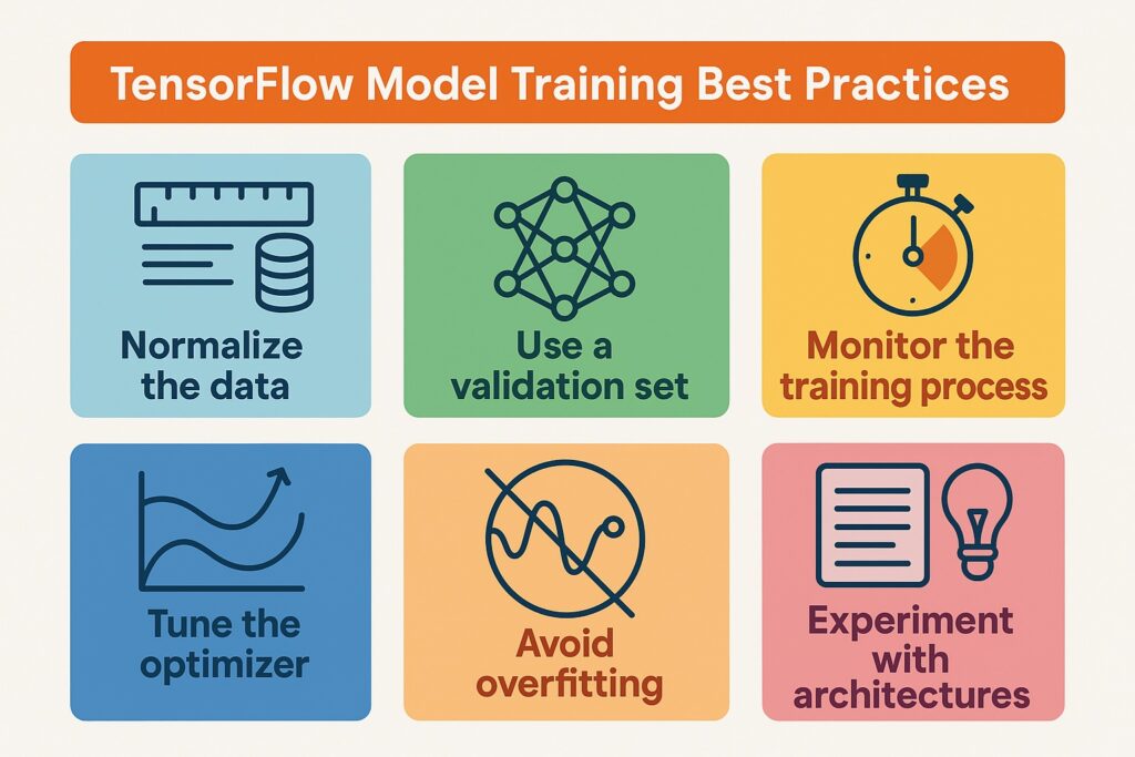
There are several best practices to consider when training models with TensorFlow, with some of them explored in our demonstration.

One of the practices we included in the demonstration was early stopping. We did this by setting up the EarlyStopping function as a callback when invoking the training function. This saves time when training cannot further reduce the loss, so there’s no point in continuing the iteration.

We also considered and implemented normalizing the input data through the normalization function. This ensured that no particular feature dominated the training and biased the model. However, it appeared that outliers were significantly skewing the data; therefore, we used the Huber function.

Another valuable practice is experimenting with learning rates to improve training and reduce the loss function. Well-tuned learning rates improve model convergence and reduce unnecessary training cycles, wasting processing resources. Also, it prevents instability during training, therefore reducing divergence risk and avoiding poor local minima.

In our demonstration, we ran the training over Apple’s M4 GPU processor, utilizing the GPU’s raw power. Because training is computationally intensive, specially designed processors like GPUs or TPUs are essential.

Setting random seeds is a useful best practice since it ensures experiments produce the same results every time for consistency. This helps with debugging and comparing models by removing randomness from training runs.

Conclusion and Next Steps

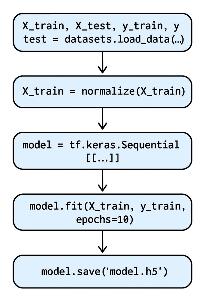
We followed several steps in training our model with TensorFlow, starting with loading California Housing data from CSV files. Next, we invoked TensorFlow’s functions for packing data to work with the model, as well as data normalization, to prevent certain features from dominating the training. We constructed the model specifying the layers and neuron density of these layers, thereby specifying the model blueprint. After specifying the model, we wired up the neurons by specifying the transfer function, the optimization algorithm, and the loss function. These were selected by invoking TensorFlow’s compile function. Once the model was wired up, we executed the training function that included the number of epochs and other tuning parameters.

The model we trained still had a high loss, indicating there was still room for improvement. Therefore, the reader can further explore model training with TensorFlow through deeper dives into hyperparameter tuning, CNNs, and TensorBoard.

The reader is encouraged to follow the example here and also apply models trained with TensorFlow to their data.

How to Train a Model with TensorFlow: Step-by-Step Guide for Beginners