Introduction
Confusion matrix explained applies to machine learning classification models that make predictions on non-deterministic data and therefore require statistical evaluation. Factors such as class imbalance and the differing costs of false positives and false negatives can significantly influence model performance. Consequently, accuracy alone is insufficient to fully evaluate a classification model. Instead, it should be complemented with additional evaluation methods that provide deeper insight into prediction outcomes.
Machine learning research has established the confusion matrix as a fundamental framework for evaluating classification models. It compares predicted labels with actual outcomes by organizing prediction results into a structured table. This enables rapid identification of correct and incorrect classifications while providing insight into the types of errors a model makes. Consequently, the confusion matrix forms the foundation for deriving widely used classification performance metrics.
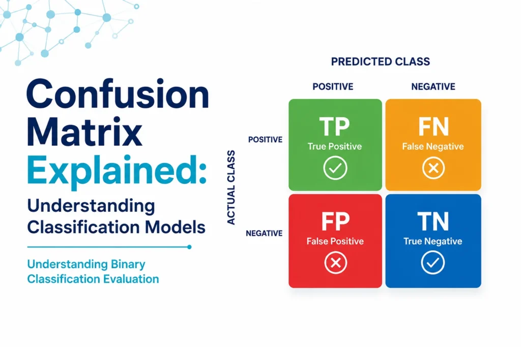
Binary classification produces four possible prediction outcomes. True Positives (TP) are instances correctly classified as positive, whereas False Positives (FP) are instances incorrectly classified as positive. True Negatives (TN) are instances correctly classified as negative, whereas False Negatives (FN) are instances incorrectly classified as negative. The confusion matrix presents these outcomes in a structured and digestible format, while metrics derived from it evaluate classifier performance, including precision, recall, accuracy, and the F1 score. These concepts are widely applied to real-world machine learning classification problems.
What Is a Confusion Matrix in Machine Learning?
A confusion matrix is a table that compares a classification model’s predicted labels with the corresponding actual labels. It summarizes classification performance and identifies prediction errors, providing insight into model effectiveness. Hence, it is an evaluation framework for classification models, in which several derived metrics describe the quality of model predictions. The confusion matrix serves as the foundation for assessing the performance of classifiers.
Machine learning classifiers operating on non-deterministic data inevitably produce some incorrect predictions. This makes the confusion matrix valuable since it allows comparison of correct and incorrect predictions and identifies prediction errors. Engineers can quantify classification results and assess classifier effectiveness. They can evaluate performance beyond accuracy, allowing them to optimize classifiers based on their use case.
The confusion matrix simplifies a classifier’s prediction results on non-deterministic data into a standard 2×2 matrix structure. The rows represent actual class labels, the columns represent the predicted class labels, and the matrix cells represent the prediction outcomes. This enables the confusion matrix to visually represent the four possible classification outcomes that is easily understood. This makes it the foundation for binary classification evaluation.
The classification outcomes presented by the confusion matrix forms the basis for classification performance metrics. The metrics derived from the classification outcomes are precision, recall, accuracy, and F1 score. They enable ML engineers to quantitatively interpret classifier behavior and evaluate prediction trade-offs based on the purpose of the classifier. ML engineers can then tune the classifier based on its performance metrics and its real-world application.
Structure of a Confusion Matrix
The confusion matrix displays binary classification outcomes, allowing engineers to identify correct classifications and misclassifications at a glance. It organizes classification outcomes into rows representing actual class labels and columns representing predicted class labels. The matrix cells represent classification outcomes that can be read quickly.
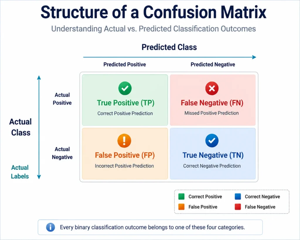
Binary classification yields four possible outcomes, shown as cells for interpretation at a glance. The first row contains cells for when the actual class labels are positive. These are True Positives (TP) in the predicted-positive column and False Negatives (FN) in the predicted-negative column. The second row contains cells for when the actual class labels are negative. These are False Positives (FP) in the predicted-positive column and True Negatives (TN) in the predicted-negative column.
True Positives (TP)
True Positives (TP) occur when both the actual value and predicted value are positive. This is when the binary classifier correctly identifies positive instances.
A real-world classification example is medical diagnosis, where the classifier correctly predicts the presence of a medical condition, resulting in treatment. This is evaluated as a true positive since both the actual and predicted values are positive.
False Positives (FP)
False Positives (FP) occur when the actual value is negative, but the predicted value is positive. In this case, the binary classifier incorrectly predicts the value as positive when it was negative.
Continuing the real-world example with medical diagnosis, the classifier incorrectly identifies a medical condition for a patient when that condition is not present. This is evaluated as a false positive because the condition is not present but is predicted to be present, resulting in unnecessary follow-up.
True Negatives (TN)
True Negatives (TN) occur when both the actual value and predicted value are negative. This is when the binary classifier correctly identifies negative instances.
For the example of medical diagnosis, the classifier identifies the absence of a medical condition for a patient when the condition is not present. This is evaluated as a true negative since both the actual and predicted values are negative, saving any unnecessary follow-up.
False Negatives (FN)
False Negatives (FN) occur when the actual value is positive, but the predicted value is negative. In this case, the binary classifier incorrectly predicts the value as negative when it was positive.
In many cases, this is the most serious situation for the medical diagnosis example. The classifier incorrectly identifies that the patient is free from a medical condition when it is present. This is evaluated as a false negative because the condition is present but predicted as not present. For certain medical conditions, this can result in serious illness or death.
How to Read a Confusion Matrix
The confusion matrix allows quick, at-a-glance interpretation of classification performance. It is intended to be read with rows and columns together, displaying the actual class labels versus the predicted class labels, similar to reading any other table.
It instantly shows the relationship between matrix cells and classification outcomes, allowing for identification of correct classifications and misclassifications. These classifications have implications for real-world decisions, including medical diagnosis, where serious medical conditions can go undetected. However, for spam email, classifying non-spam email as spam can be frustrating.
Reading a Confusion Matrix Example
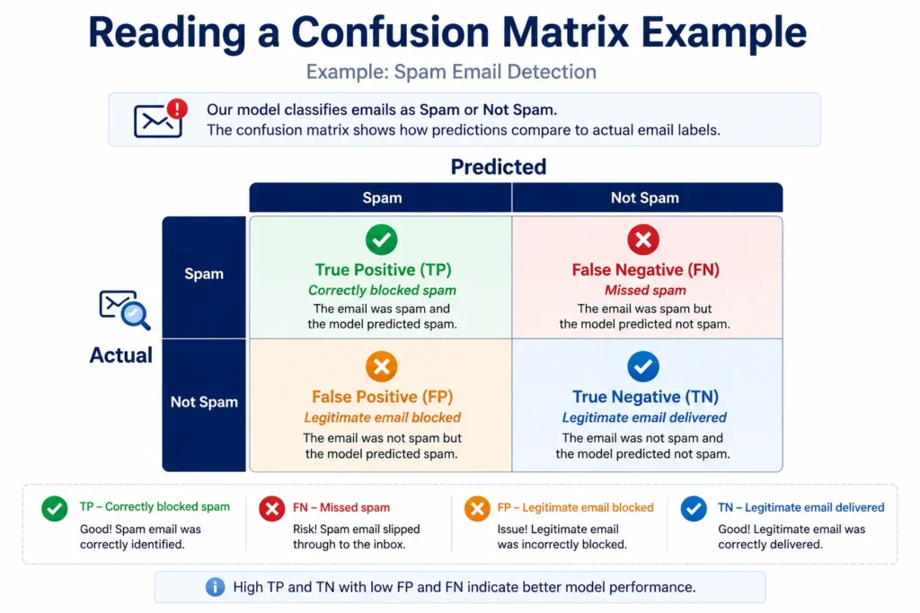
A common example is spam email classification, which illustrates how to use the confusion matrix. Here, the positive class is that the email is spam, while the negative class is that the email is not spam. The rows represent whether the email is spam or not spam, while the columns represent whether it was classified as spam or not.
TP is when it was correctly classified as spam, and FN is when it was incorrectly classified as not spam. FP is when it was incorrectly classified as spam, and TN is when it was correctly classified as not spam. Additionally, the confusion matrix shows the distribution of prediction outcomes across the two classes. This provides insight into the classification algorithm’s performance.
Real-World Interpretation
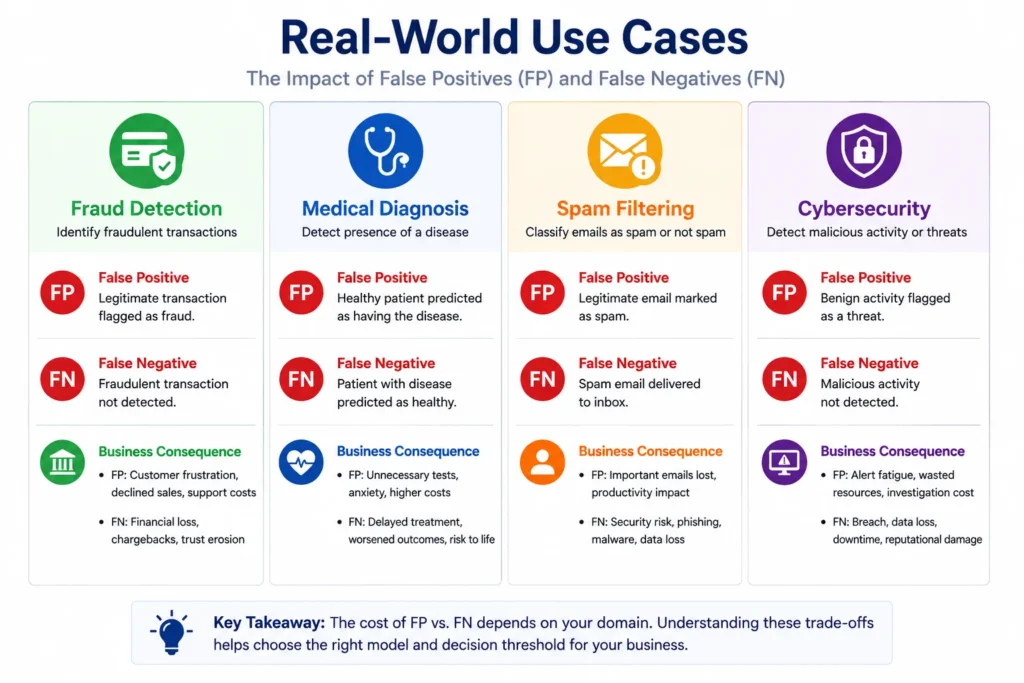
Credit card fraud detection is an important example of binary classification used by all financial institutions. The positive class represents fraudulent transactions, while the negative class represents legitimate transactions. There is a direct business impact of misclassifications. FN represents fraudulent transactions classified as legitimate, resulting in financial loss. FP represents legitimate transactions that are classified as fraudulent, adding operational overhead and customer frustration.
Medical diagnosis is another important example of binary classification used extensively throughout health care. The prediction outcomes lead to decisions about next steps by health care professionals. FPs are nonexistent health conditions that are incorrectly diagnosed, leading to unnecessary additional medical activity and costs. FNs are missed health conditions that lead to delayed treatment and potentially worsen patient outcomes. It is important to balance these classification errors where derived metrics are needed.
Why Confusion Matrices Matter
Examples like fraud detection and medical diagnosis clearly illustrate that misclassifications have serious repercussions. This makes it essential to understand the distribution of misclassifications, since accuracy alone is insufficient. Evaluating classification performance requires a comprehensive assessment.
Binary classification has two types of prediction errors. The first is when classification predicts the item as negative when it is actually positive (False Negative). The other is when an item is predicted as positive even though it is actually negative (False Positive). Confusion matrices provide deeper insight into this behavior.
Beyond Accuracy
Accuracy does not include the misclassification distributions needed to optimize real-world scenarios. It is misleading since certain misclassifications may have serious repercussions that accuracy does not capture. When evaluating classification performance, it is necessary to consider all prediction outcomes rather than relying on accuracy alone. Engineers should have visibility into both correct and misclassified cases.
Datasets used to train classification algorithms are often imbalanced due to the characteristics of the environments they represent. Classification accuracy can mask the performance of minority classes, yielding an incorrect evaluation of classification performance. This highlights the importance of False Positives and False Negatives, as well as the need for confusion matrix analysis.
Understanding Prediction Errors
Evaluating classifier performance includes understanding prediction error, and the first stage is visibility into False Positives and False Negatives. Engineers should identify patterns of prediction error to improve their interpretation of classification behavior. This allows them to identify sources of systematic classification errors, thereby supporting classifier optimization and improvement.
While the confusion matrix reveals patterns in prediction errors, it does not explain which input variables are influencing the model’s decisions. Feature importance in machine learning provides this complementary perspective by identifying the features that have the greatest influence on model behavior.
Confusion matrices provide visibility to these errors but also serve as the basis for derived evaluation metrics. Metrics derived from prediction outcomes include precision, recall, accuracy, and F1 scores. These metrics provide further insight into classification performance and typically present trade-offs among them during classification optimization. Each metric is typically more relevant to certain real-world problems than others.
Confusion Matrix and Classification Metrics
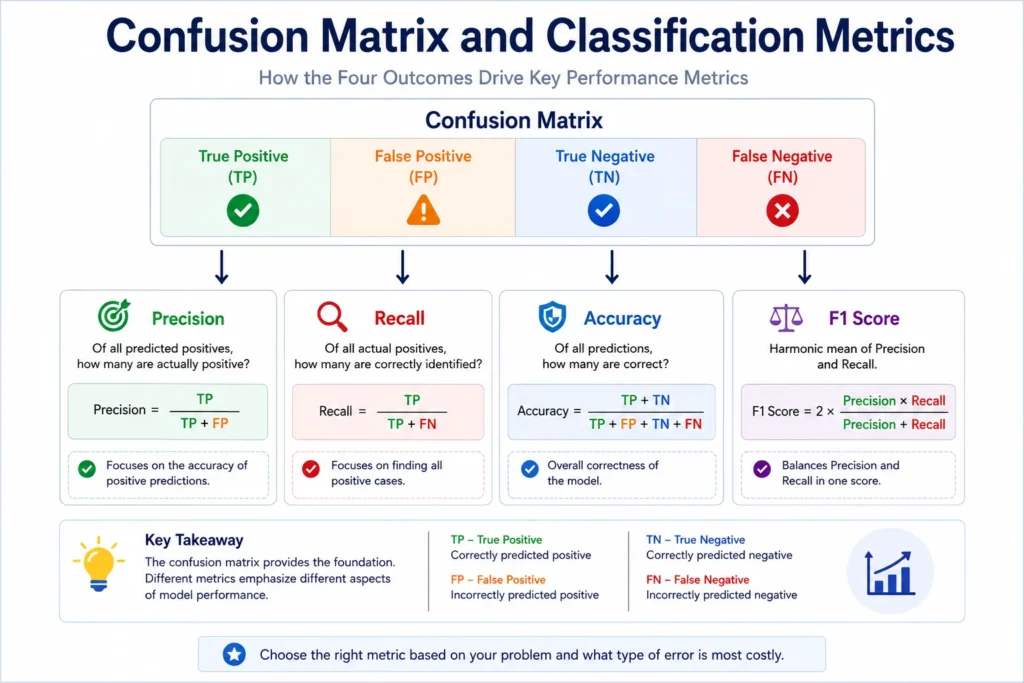
The confusion matrix serves as the basis for classification evaluation since it displays the distribution of correct and incorrect classifications. However, metrics derived from these classification outcomes provide a more meaningful assessment of classifier performance aligned with real-world use cases.
Each of these derived metrics emphasizes different prediction outcomes, and no single metric is suitable for every classification problem. Selection of metrics is based on real-world problems for which they are suited to optimize the classification algorithm in that domain.
Precision
Precision is a derived metric that focuses on positive predictions made by the classifier. It indicates the proportion of positive predictions that are correctly classified and is derived from True Positives (TP) and False Positives (FP). Its formula is:
Precision = TP / (TP + FP)
It measures prediction correctness for positive predictions.
False Positives are often termed as false alarms, and Precision is important when these false alarms are costly. Two examples are spam email classification and credit card fraud detection. Engineers use Precision to tune classification algorithms to reduce False Positives or false alarms.
Recall
Recall is a derived metric that focuses on actual positive instances identified by the classifier. It indicates the proportion of actual positives that are correctly classified and is derived from True Positives (TP) and False Negatives (FN). Its formula is:
Recall = TP / (TP + FN)
It measures positive instance detection for actual positives.
For certain classes of real-world examples, Recall is important when False Negatives are costly. Medical diagnosis is an important example of this. False Negatives correspond to missed diagnosis of serious health conditions, delaying treatment. Engineers use Recall to tune classification algorithms to reduce False Negatives.
Accuracy
Accuracy is also a derived metric that focuses on the overall performance of the classifier. It indicates the proportion of correctly classified instances and is derived from all classified instances. Its formula is:
Accuracy = (TP + TN) / (TP + FP + FN + TN)
It measures the overall proportion of correctly classified instances.
Although other metrics are needed, it is still highly applicable for balanced datasets. However, it is limited for imbalanced datasets since it masks minority-class performance. Engineers use Accuracy to tune classification algorithms that are applied to balanced datasets.
F1 Score
This metric is a secondary derived metric that is derived from precision and recall and measures the relationship between these two. It measures the harmonic mean between precision and recall, and its formula is:
F1 Score = 2 x (Precision x Recall) / (Precision + Recall)
It is a balanced summary of precision and recall
There are many classes of problems where both precision and recall are important, and it is also important for imbalanced domains. Engineers use the F1 score to improve both Precision and Recall in classification algorithms.
Real-World Use Cases
There are many real-world use cases that involve binary classification for either manual or automated decision-making. Misclassifications have important consequences, making it necessary to understand the distribution of misclassifications when evaluating and refining binary classifiers.
There are different types of prediction errors, and each real-world use case is impacted differently by them. The confusion matrix presents the distribution of prediction errors, allowing engineers to optimize classifiers based on prediction error prioritization.
Business and Financial Applications
Credit card transactions are a core function of the modern economy, with credit card fraud incurring major financial and reputational costs. Therefore, fraud detection is an essential activity in classifying fraudulent and non-fraudulent transactions. However, there is a trade-off between fraud prevention (reducing False Negatives) and customer experience (reducing False Positives). The confusion matrix is used to optimize these conflicting business objectives.
Emails have been embedded in daily life for several decades, with spam email impacting business productivity and user experience. Email providers universally perform spam email filtering using binary classification of spam and legitimate email. Prediction error trade-offs involve balancing between blocked spam and legitimate email delivery. The confusion matrix is used to optimize email filtering.
Healthcare and Cybersecurity Applications
Healthcare is invariably overwhelmed by patient health data when making diagnoses, and automated diagnostic tools are long-established. These tools are classifiers that make a binary classification of the presence or absence of health conditions. Missed diagnoses correspond to False Negatives and can make the health condition far more serious due to delayed treatment. Confusion matrices are invariably used to support healthcare decision-making by reducing False Negatives or missed diagnoses.
IT is the fundamental layer of all modern society, and cyberattacks can have potentially grave consequences. Cybersecurity alert detection is an active and fundamental layer of defense against cyberattacks. It classifies events as either malicious or benign. However, both missed threats (False Negatives) and false alerts (False Positives) are serious, with false alerts leading to alert fatigue. Therefore, the confusion matrix is used to optimize cybersecurity detection systems by simultaneously reducing missed threats and false alerts.
Common Mistakes When Interpreting a Confusion Matrix
Accuracy and Class Imbalance
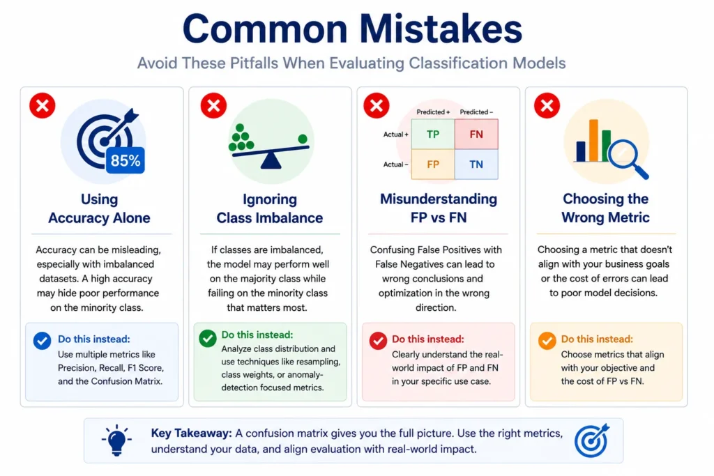
The most fundamental mistake when interpreting a confusion matrix is relying solely on accuracy for evaluating classifiers. It overlooks the distribution of prediction outcomes when misclassifications may have significant consequences for the particular use case. This makes it important to include all confusion matrix outcomes when evaluating classifiers.
The domains of many use cases are often skewed to one outcome over the other, resulting in a class imbalance during classifier evaluation. Relying on accuracy masks the performance of the minority class, making the binary classifier flawed. The confusion matrix, along with False Positives and False Negatives, is needed to reveal minority-class prediction errors.
Prediction Errors and Metric Selection
After relying on accuracy alone, the other key mistake is misunderstanding the trade-offs between the two types of misclassifications. Different applications prioritize the different prediction errors of False Positives and False Negatives. Therefore, the selection of evaluation metrics must be based on the business and operational impact of prediction errors.
Additionally, engineers can choose an evaluation metric that does not align with the real-world use case. Since different applications prioritize different prediction errors, engineers must select the metric that best aligns with the application’s objectives. For example, choosing Precision over Recall for medical diagnosis could increase missed diagnoses, leading to serious consequences for patients.
Hence, it is important to avoid reliance on a single evaluation metric for a problem as simple as binary classification. It is important to interpret both raw and derived metrics along with the application context when evaluating and optimizing classifiers. Therefore, engineers should combine confusion matrix insights with derived evaluation metrics.
Final Thoughts
The confusion matrix serves as the foundation for evaluating and optimizing binary classifiers for a wide range of real-world problems. It tabulates a summary of classification outcomes, enabling engineers to interpret classifier behavior. Engineers can understand correct classifications and misclassification distributions at a glance, which are important for understanding classifier behavior.
The confusion matrix provides raw metrics of binary classifier performance, but there are also metrics derived from these raw metrics. They are precision, recall, accuracy, and F1 score, and are typically aligned with use-case prioritization rather than raw metrics. Classifier optimization relies on the selection of evaluation metrics based on application requirements.
Overall, this makes the confusion matrix an essential tool for machine learning evaluation. The raw metrics it presents, along with the derived metrics, enable engineers to build reliable, application-specific classification models. The reader is encouraged to further explore related classification evaluation topics, including Precision vs. Recall, AUC vs. F1 Score, and ROC Curve vs. Precision–Recall Curve.
References
scikit-learn — Evaluate the performance of a classifier with Confusion Matrix
scikit-learn — Metrics and scoring: quantifying the quality of predictions
Google Developers Guide — Classification: Accuracy, recall, precision, and related metrics
Microsoft Learn — Evaluation Metrics
Recommended Books
Pattern Recognition and Machine Learning – Christopher M. Bishop
Excellent graduate-level reference covering probabilistic classification, evaluation metrics, Bayesian learning, and statistical machine learning.
Hands-On Machine Learning with Scikit-Learn, Keras, and TensorFlow: Concepts, Tools, and Techniques to Build Intelligent Systems – Aurélien Géron
Practical machine learning guide with extensive coverage of classification algorithms, confusion matrices, precision, recall, ROC curves, and model evaluation.
An Introduction to Statistical Learning: with Applications in Python – Gareth James
Accessible introduction to statistical learning with practical examples and model evaluation techniques.
Recommended Training
Build practical skills in machine learning classification, model evaluation, feature engineering, and scikit-learn implementation through expert-led Pluralsight courses.
Affiliate Marketing Disclosure
Some of the links on this page are affiliate links. As an Amazon Associate, AI Cloud Data Pulse earns from qualifying purchases. We may also earn commissions through other affiliate programs, including Pluralsight, at no additional cost to you. We only recommend books, training, and resources that we believe provide genuine educational value to machine learning practitioners.